Vectorial Optical Transfer Function
Analysing the spatial frequencies in high aperture imaging.
This web page is based on:Matthew R. Arnison and Colin. J. R. Sheppard, A 3D vectorial optical transfer function suitable for arbitrary pupil functions, Optics Communications, 211, 53-63 (2002).
The point spread function (PSF) is the electric field in the focal region of a lens. The optical transfer function (OTF) is simply the Fourier transform of the intensity of the PSF. Like any Fourier transform, it can be used to describe the spatial frequency content of the PSF. This is useful when analysing an imaging system to predict which coarse and fine features will be successfully imaged.
For high resolution imaging, we need to use high aperture lenses, where the light converges from a wide angle onto the focal region. This means the small angle approximation (also known as the paraxial approximation) is no longer valid. It also means that the scalar approximation (which assumes that the electric field is scalar rather than vectorial) becomes increasingly inaccurate.
So when we model high aperture lenses, we use the vectorial PSF and the vectorial OTF for best accuracy.
However, while the vectorial PSF has been studied for decades, the vectorial OTF is a relatively new concept. Previous high aperture OTF models have assumed the imaging system does not change with rotation about the imaging axis (radially symmetric).
Recently we published a method for calculating the vectorial OTF which does not assume any radial symmetry in the imaging system. This allows us to properly model the vectorial nature of the light when the input is a plane polarised beam. It also allows the modeling of arbitrary imaging aberrations.
We start with the vectorial pupil function Q(m,n,s) which is defined on the surface of the cap of a sphere:
We could find the OTF by doing a 3D Fourier transform to get the PSF E(x,y,z), taking the intensity |E|^2, and then doing the inverse Fourier transform to get the OTF C(m,n,s).
An alternative approach is to use the Fourier convolution theorem to instead calculate the OTF using an auto-correlation of the pupil Q(m,n,s), to get the OTF C(m,n,s) directly.
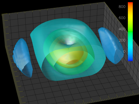
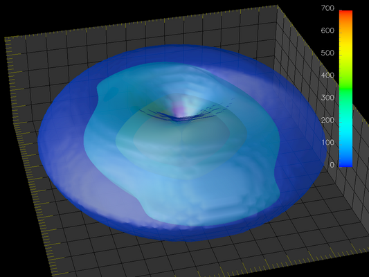
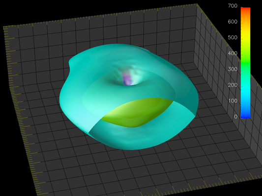
Either way, the 3D OTF looks like a dougnut:
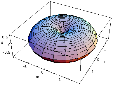
Outside the doughnut, the OTF is zero: this doughnut surface gives the maximum spatial frequencies which can be imaged using the system.
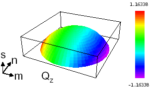
We can then slice through this doughnut to reveal the strength of the OTF for any spatial frequency (m,n,s) inside. Here m,n,s are the spatial frequencies in the x,y,z directions, respectively.
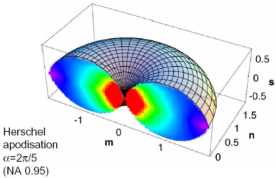
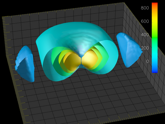
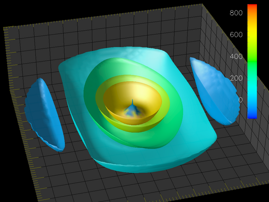
3D functions like this OTF take a little work to visualise effectively. Another way to look at the OTF is to plot iso-surfaces, which are surfaces on constant value. Iso-surfaces are the 3D equivalent of 2D contour lines.
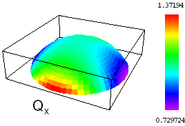
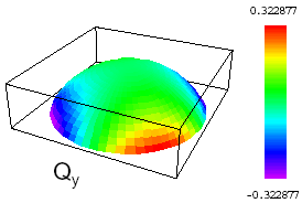
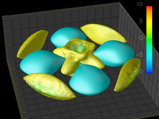
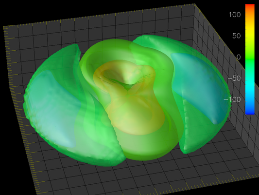
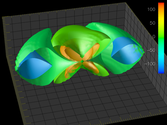
In the column on the right, we show iso-surfaces for the vectorial OTF C(m,n,s), followed by the iso-surfaces for the contributions to the OTF from the x,y,z components of the electric field in the focal region.
Note that C, Cy, and Cz are negative at high |m|. This indicates there will be a contrast reversal for objects in the specimen which have large spatial frequencies parallel to the polarisation of the input beam.
See also:
- a recent talk on this topic:
M. R. Arnison and C. J. R. Sheppard, Three dimensional optical transfer functions for high aperture systems with non-symmetric pupils, Australian Optical Society Conference, (Sydney, Australia, 2002).
- Matthew R. Arnison and Colin. J. R. Sheppard,
A 3D vectorial
optical transfer function suitable for arbitrary pupil functions,
Optics Communications, 211, 53-63 (2002).
- Matthew R. Arnison home page
Vectorial OTF iso-surfaces (click to expand or scroll down for more)
Microscope
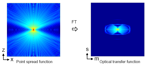
PSF and OTF
(approximate projections)
VOTF iso-surfaces:
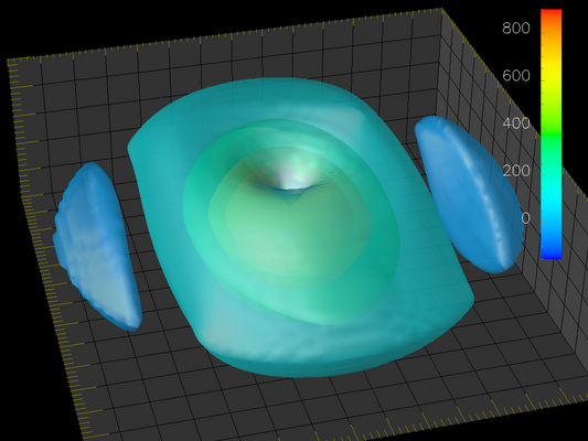
C
C
C
C
Cx
Cx
Cy
Cz
Cz